Plotting

StatsPlots

JuliaDB has all access to all the power and flexibility of Plots via StatsPlots and the @df macro.

using JuliaDB, StatsPlots

t = table((x = randn(100), y = randn(100)))

@df t scatter(:x, :y)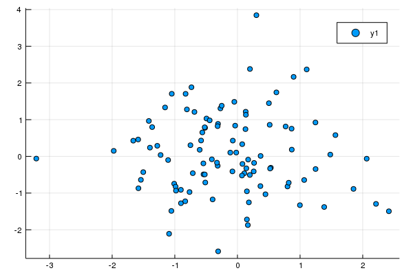

Plotting Big Data

For large datasets, it isn't feasible to render every data point. The OnlineStats package provides a number of data structures for big data visualization that can be created via the reduce and groupreduce functions.

• Example data:

using JuliaDB, Plots, OnlineStats

x = randn(10^6)
y = x + randn(10^6)
z = x .> 1
z2 = (x .+ y) .> 0
t = table((x=x, y=y, z=z, z2=z2))

Table with 1000000 rows, 4 columns:
x           y           z      z2
────────────────────────────────────
1.48494     2.19288     true   true
1.23969     0.536499    true   true
1.06159     1.42904     true   true
0.176156    0.249636    false  true
0.714251    -0.0450475  false  true
-0.0682377  -1.35414    false  false
0.05331     -0.823936   false  false
1.86        1.45448     true   true
0.855915    2.66493     false  true
⋮
-1.75701    -0.285743   false  false
0.356983    -0.459484   false  false
-1.13729    -0.7288     false  false
1.82383     2.88267     true   true
-1.57593    -2.79145    false  false
-1.93871    -0.447352   false  false
-0.800527   -0.392614   false  false
-0.384413   -2.00444    false  false

Mosaic Plots

A mosaic plot visualizes the bivariate distribution of two categorical variables.

o = reduce(Mosaic(Bool, Bool), t; select = (3, 4))
plot(o)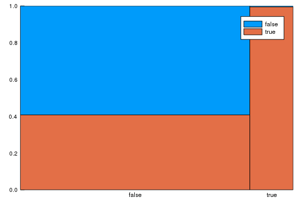

Histograms

grp = groupreduce(Hist(-5:.5:5), t, :z, select = :x)
plot(plot.(select(grp, 2))...; link=:all)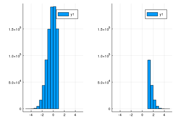

grp = groupreduce(KHist(20), t, :z, select = :x)
plot(plot.(select(grp, 2))...; link = :all)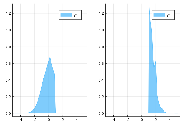

Partition and IndexedPartition

• Partition(stat, n) summarizes a univariate data stream.
  • The stat is fitted over n approximately equal-sized pieces.
• IndexedPartition(T, stat, n) summarizes a bivariate data stream.
  • The stat is fitted over n pieces covering the domain of another variable of type T.

o = reduce(Partition(KHist(10), 50), t; select=:y)
plot(o)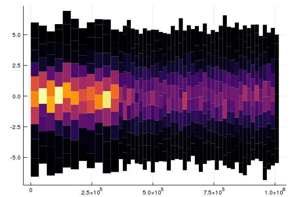

o = reduce(IndexedPartition(Float64, KHist(10), 50), t; select=(:x, :y))
plot(o)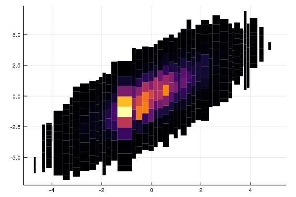

GroupBy

o = reduce(GroupBy{Bool}(KHist(20)), t; select = (:z, :x))
plot(o)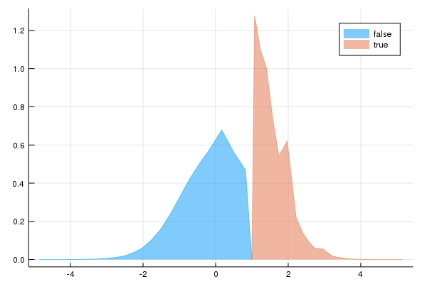

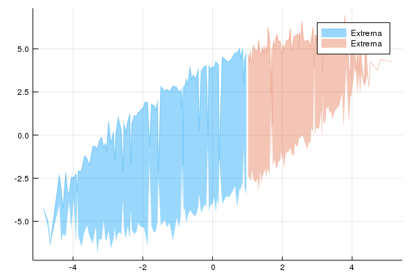
Convenience function for Partition and IndexedPartition

You can also use the partitionplot function, a slightly less verbose way of plotting Partition and IndexedPartition objects.

# x by itself
partitionplot(t, :x, stat = Extrema())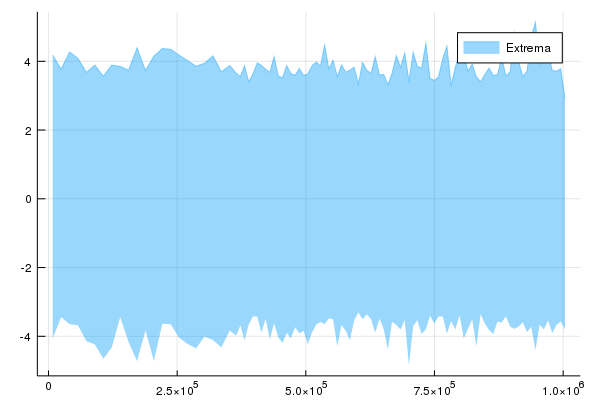

# y by x, grouped by z
partitionplot(t, :x, :y, stat = Extrema(), by = :z)